Reconstructing Phenotype-Specific Single-Omics Networks with SmCCNet

SmCCNet package

The SmCCNet package has the following dependencies:

library(pbapply)
library(Matrix)
library(igraph)
library(SmCCNet)
library(parallel)

This section provides a tutorial on running the SmCCNet algorithm for a quantitative phenotype using single-omics data. Please see other vignettes for multi-omics applications.

SmCCNet single-omics workflow with a synthetic dataset

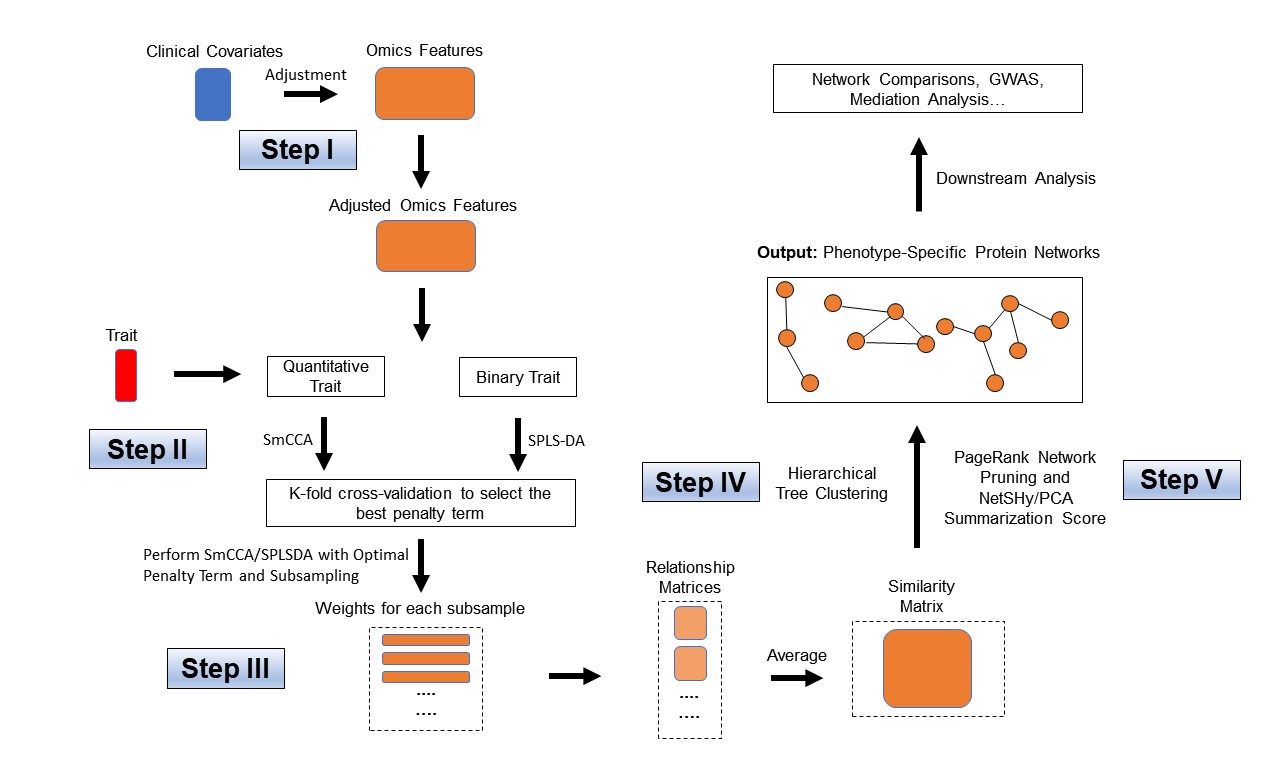
Workflow for SmCCNet single-omics setting (binary and quantitative phenotype).

As an example, we consider a synthetic data set with 500 genes \((X_1)\) expression levels measured for 358 subjects, along with a quantitative phenotype \((Y)\). The example has a single phenotype, but a multi-dimensional phenotype matrix is also possible.

data(ExampleData)
head(X1[ , 1:6])

##          Gene_1   Gene_2   Gene_3   Gene_4   Gene_5   Gene_6
## Samp_1 22.48570 40.35372 31.02575 20.84721 26.69729 30.20545
## Samp_2 37.05885 34.05223 33.48702 23.53146 26.75463 31.73594
## Samp_3 20.53077 31.66962 35.18957 20.95254 25.01883 32.15723
## Samp_4 33.18689 38.48088 18.89710 31.82330 34.04938 38.79989
## Samp_5 28.96198 41.06049 28.49496 18.37449 30.81524 24.00454
## Samp_6 18.05983 29.55471 32.54002 29.68452 26.19996 26.76684

head(Y)

##           Pheno
## Samp_1 235.0674
## Samp_2 253.5450
## Samp_3 234.2050
## Samp_4 281.0354
## Samp_5 245.4478
## Samp_6 189.6231

Denote the number of features in \(X_1\) as \(p_1\) and the number of subjects as \(n\).

p1 <- ncol(X1)
N <- nrow(X1)
AbarLabel <- colnames(X1)

Step I. Preprocessing

The first step is to preprocess the single omics data. All canonical correlation analysis (CCA) methods require data sets to be standardized (centered and scaled) by columns (e.g. features) to ensure the equivalent contribution of each feature when maximizing covariance. In addition, there are some other optional steps to preprocess the data. Note that when employing both standardization and covariate adjustment, it is essential to apply standardization prior to covariate adjustment. This sequencing ensures our best efforts to meet the assumptions of linear regression In our data preprocessing pipeline, the following options are given (with ordering):

1. CoV Filtering: Filter features based on coefficients of variation (CoV).
2. Standardization: Center and/or scale data.
3. Adjust for Covariates: Regress out specified covariates and return residuals

Below is an example of data preprocessing with only feature filtering and standardization, in this case, there is no covariate adjustment, the coeffcient of variation filtering quantile is 0.2 (meaning that features with CoV smaller than 20% quantile of CoV will be filtered out), and data are centered and scaled:

# preprocess data
processed_data <- dataPreprocess(X = as.data.frame(X1), covariates = NULL, 
                  is_cv = TRUE, cv_quantile = 0.2, center = TRUE, scale = TRUE)

Step II: Determine optimal sparsity penalties through cross-validation (optional)

To find the optimal sparsity penalties, we apply a K-fold cross-validation on the synthetic data (Figure 1). Let \(p_1\) denote the number of features in omics data \(X_1\) respectively, and \(s_1\) is the proportion of \(X_1\) features to be sampled every time. The sparse penalties range from 0.05 to 0.3 with step size of 0.05. Large penalty values correspond to less sparse canonical weight vector, while small penalties correspond to sparser canonical weight vector. Below is the list of parameters that need to be specified:

\(K\): Number of folds in cross-validation (CV). Typically a 5-fold CV is sufficient. If the training set contains too few (e.g. \(<30\)) samples, or the test or training set becomes unscalable, then choose a smaller \(K\).

K <- 3 # number of folds in K-fold CV.
s1 <- 0.7
subSamp <- 50 # number of subsamples (will be described in later section).

# create sparsity penalty options.
pen1 <- seq(.05, .3, by = .05)

# set a CV directory.
CVDir <- "Example3foldCV/" 
pheno <- "Example3foldCV"
dir.create(CVDir)

Create test and training data sets.

To perform K-fold Cross-Validation (CV), we need to split the data (\(X_1, Y\)) into test and training sets. We have included the standardization step within the SmCCNet algorithm. However, for the CV procedure, we recommend to standardize the training and test sets upfront, since this helps to choose the number of CV folds \(K\). If any data set can not be standardized, we recommend to reduce \(K\). In the code below, we show how to create CV data sets and check if all data sets are valid (i.e. standardizable). The standardized training and test data sets will be saved under the CV directory.

# set random seed
set.seed(12345) 

# save data and parameters into local directory
save(X1, Y, s1, subSamp, pen1, 
     file = paste0(CVDir, "Data.Rdata"))

# split data into K folds
foldIdx <- split(1:N, sample(1:N, K))
for(i in 1:K){
  iIdx <- foldIdx[[i]]
  x1.train <- scale(X1[-iIdx, ])
  yy.train <- Y[-iIdx, ]
  x1.test <- scale(X1[iIdx, ])
  yy.test <- Y[iIdx, ]
  
  if(is.na(min(min(x1.train), min(yy.train), min(x1.test), min(yy.test)))){
    stop("Invalid scaled data.")
  }
  
  subD <- paste0(CVDir, "CV_", i, "/")
  dir.create(subD)

  # save data from each fold into local directory
  save(x1.train, yy.train, x1.test, yy.test,
       pen1, p1, 
       file = paste0(subD, "Data.Rdata"))
}

Run K-fold Cross-Validation

For each of the K-folds, we compute the prediction error for each penalty pair option. Since there is no subsampling step for cross-validation, we run through cross-validation with nested for loop. However, if the omics data are extremely high-dimensional, we recommend using the R package parallel to parallelize the for loop, or use fastAutoSmCCNet() directly. fastAutoSmCCNet() is the package built-in function that streamline the pipeline with single line of code, and the cross-validation step is parallelized with the future_map() in furrr package.

# number of clusters in parSapply should be the same as number specified above
suppressWarnings(for (CVidx in 1:K)
{
  # define the sub-directory for each fold 
  subD <- paste0(CVDir, "CV_", CVidx, "/")
  # load fold data
  load(paste0(subD, "Data.Rdata"))
  dir.create(paste0(subD, "SmCCA/"))
  # create empty vector to store cross-validation result
  RhoTrain <- RhoTest <- DeltaCor <- rep(0, length(pen1))
  # evaluate through all the possible penalty candidates
  for(idx in 1:length(pen1)){
    l1 <- pen1[idx]
    print(paste0("Running SmCCA on CV_", CVidx, " pen=", l1))
    # run single-omics SmCCNet
    Ws <- getRobustWeightsSingle(x1.train, as.matrix(yy.train), l1, 1,
                                    SubsamplingNum = 1)
    # average
    meanW <- rowMeans(Ws)
    v <- meanW[1:p1]
    
    rho.train <-  cor(x1.train %*% v, yy.train)
    
    
    rho.test <- cor(x1.test %*% v, yy.test) 
    
    
    RhoTrain[idx] <- round(rho.train, digits = 5)
    RhoTest[idx] <- round(rho.test, digits = 5)
    DeltaCor[idx] <- abs(rho.train - rho.test)
    
   
    
  }
  
  DeltaCor.all <- cbind(pen1, RhoTrain, RhoTest, DeltaCor)
  colnames(DeltaCor.all) <- c("l1", "Training CC", "Test CC", "CC Pred. Error")
  write.csv(DeltaCor.all,
            file = paste0(subD, "SmCCA/SCCA_", subSamp,"_allDeltaCor.csv"))
  
  
})

Extract penalty term with the smallest total prediction error

We extract the total prediction errors and return the best penalty term. This step will automatically give the optimal testing canonical correlation choice as well as prediction error choice, which serves as a reference for the penalty term selection. There are different ways to select the best penalty terms, one of the simplest way is to minimize discrepancy between the training canonical correlation and the testing canonical correlation. However, this method does not take the magnitude of testing canonical correlation into account, which means it may end up selecting the penalty term with smaller canonical correlation (low signal). For instance, if a certain penalty term yields the training canonical correlation of 0.7, with the testing canonical correlation of 0.4, and another penalty term yield the training canonical correlation of 0.4, with the testing canonical correlation of 0.2, minimizing training and testing canonical correlation selects the latter. Therefore, in this step, we want to minimized the scaled prediction error, which is defined as:

\[\begin{equation} scaledPredErr = \frac{|trainCC - testCC|}{|testCC|}, \end{equation}\]

where \(trainCC\) and \(testCC\) is defined as the training canonical correlation and testing canonical correlation respectively.

# combine prediction errors from all K folds and compute the total prediction
# error for each sparsity penalty pair.
aggregateCVSingle(CVDir, "SmCCA", NumSubsamp = subSamp, K = K)

Step III: Run SmCCA with pre-selected penalty term

With a pre-selected penalty term, we apply SmCCA to subsampled features of \(X_1\) and \(Y\), and repeat the process to generate a robust similarity matrix (Figure 1). As for the number of subsample, a larger number of subsamples leads to more stable results, while a smaller number of subsample is faster computationally. We use 50 in this example. Below is the setup and description of the subsampling parameters:

\(s1\): Proportions of feature subsampling from \(X_1\). Default values are \(s_1 = 0.7\).
\(SubsamplingNum\): Number of subsamples.

After obtaining the canonical weight \(Ws\), which has the dimension of \(p_1\) (number of features) by \(p_1 s_1\) (proportion of feature subsamples), the next step is to obtain the adjacency matrix by taking the outer product of each \(W\) with itself to obtain an adjacency matrix and average the matrices to obtain \(Abar\), a sparse matrix object.

# set up directory to store all the results
plotD <- paste0(CVDir, "Figures/")
saveD <- paste0(CVDir, "Results/")
dataF <- paste0(CVDir, "Data.Rdata")
dir.create(plotD)
dir.create(saveD)
dir.create(dataF)

# type of CCA result, only "SmCCA" supported
Method = "SmCCA"


# after SmCCA CV, select the best penalty term, 
# and use it for running SmCCA on the complete dataset
for(Method in "SmCCA"){
  # select optimal penalty term from CV result
  T12 <- read.csv(paste0(CVDir, "Results/", Method, "CVmeanDeltaCors.csv"))
  # calculate evaluation metric **
  pen <- T12[which.min(T12[ ,4]/abs(T12[ ,3])) ,2]
  
  
  l1 <- pen;
  system.time({
    Ws <- getRobustWeightsSingle(X1 = X1, Trait = as.matrix(Y), 
                                       Lambda1 = l1, 
                                       s1, SubsamplingNum = subSamp)
    
    
    Abar <- getAbar(Ws, FeatureLabel = AbarLabel[1:p1])
    save(l1, X1, Y, s1, Ws, Abar,
         file = paste0(saveD, Method, K, "foldSamp", subSamp, "_", pen, 
                       ".Rdata"))
  })
  
  
}

Step IV: Obtain single-omics modules through network clustering

From the similarity matrix obtained in the last step, we obtain single-omics modules by applying hierarchical tree cutting and plotting the reconstructed networks. The edge signs are recovered from pairwise feature correlations.

# perform clustering based on the adjacency matrix Abar 
OmicsModule <- getOmicsModules(Abar, PlotTree = FALSE)

# make sure there are no duplicated labels
AbarLabel <- make.unique(AbarLabel)

# calculate feature correlation matrix
bigCor2 <- cor(X1)

# data type
types <- rep('gene', nrow(bigCor2))

Step V: Obtain network summarization score and pruned subnetworks

The next step is to prune the network so that the unnecessary features (nodes) will be filtered from the original network module. This principle is based on a subject-level score of interest known as the network summarization score. There are two different network summarization methods: PCA and NetSHy (network summarization via a hybrid approach, Vu et al 2023 Bioinformatics), which are specified by the argument ‘method’. We evaluate two criteria stepwise 1) summarization score correlation with respect to the phenotype, which is used to verify if the summarization score for the current subnetwork has a strong signal with respect to the phenotype and 2) The correlation between the summarization of the current subnetwork and that of the baseline network with a pre-defined baseline network size. This is used to check if the addition of more molecular features introduces noise. The stepwise approach for network pruning is:

Users can prune each network module obtained through hierarchical clustering with the following code:

# filter out network modules with insufficient number of nodes
module_length <- unlist(lapply(OmicsModule, length))
network_modules <- OmicsModule[module_length > 10]
# extract pruned network modules
for(i in 1:length(network_modules))
{
  cat(paste0('For network module: ', i, '\n'))
  # define subnetwork
  abar_sub <- Abar[network_modules[[i]],network_modules[[i]]]
  cor_sub <- bigCor2[network_modules[[i]],network_modules[[i]]]
  # prune network module
  networkPruning(Abar = abar_sub,CorrMatrix = cor_sub, 
                          type = types[network_modules[[i]]], 
                 data = X1[,network_modules[[i]]],      
              Pheno = Y, ModuleIdx = i, min_mod_size = 10, 
                          max_mod_size = 100, method = 'PCA', 
                          saving_dir = getwd())
  cat("\n")
}

The output from this step contains a network adjacency matrix, summarization scores (first 3 PCs), PC loadings and more, which are stored in a .Rdata file in the user-specified location.

Results

We present the single-omics network result based on the synthetic data. The first table below contains the individual molecular features correlation with respect to phenotype, and their associated p-value (from correlation testing).

Individual molecular features correlation table with respect to phenotype (correlation and p-value).
Molecular Feature	Correlation to Phenotype	P-value
Gene_1	0.3828730	0.0000000
Gene_2	0.3411378	0.0000000
Gene_5	0.1310036	0.0131111
Gene_6	0.6284530	0.0000000
Gene_7	0.6531262	0.0000000
Gene_28	0.1306018	0.0133961
Gene_46	0.1204872	0.0226039
Gene_54	-0.1385489	0.0086656
Gene_72	-0.1274960	0.0157889
Gene_74	-0.1401523	0.0079155
Gene_88	0.1234406	0.0194714
Gene_174	-0.1272991	0.0159525
Gene_189	-0.1462271	0.0055715
Gene_190	-0.1443251	0.0062277
Gene_222	0.1258673	0.0171873
Gene_367	0.1499230	0.0044714

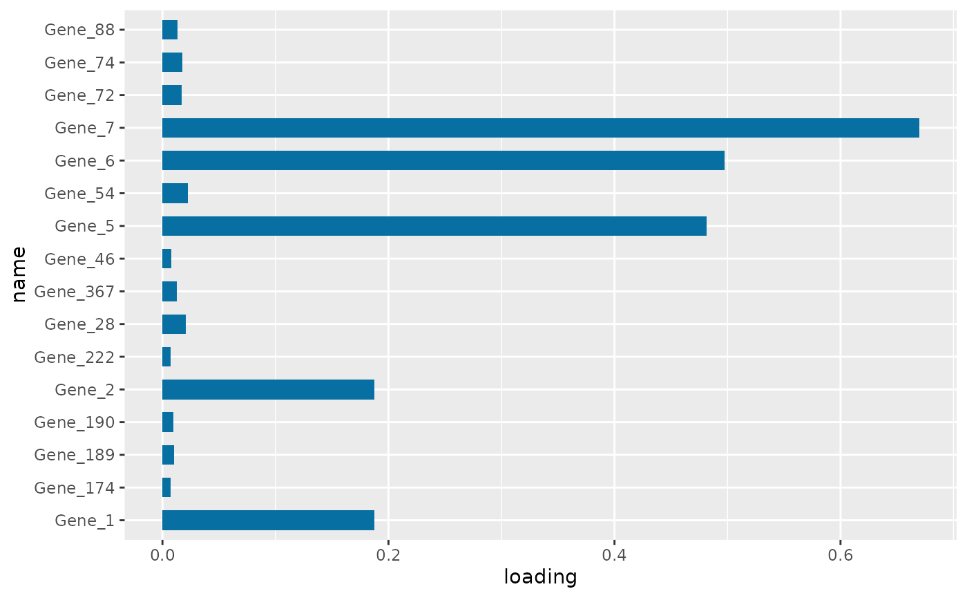
PC1 loading for each subnetwork feature.

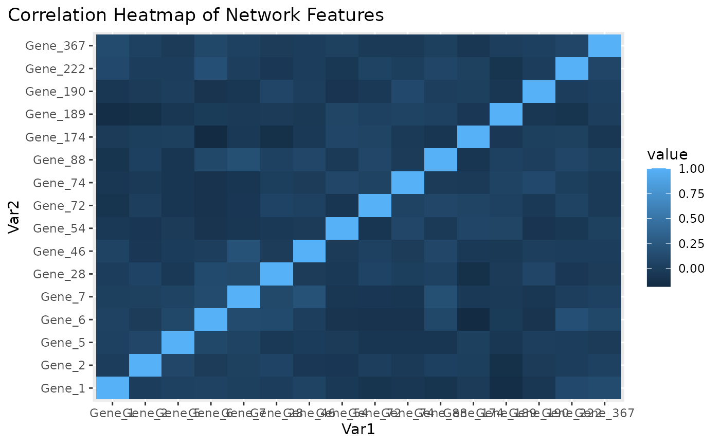
Correlation heatmap for subnetwork features.

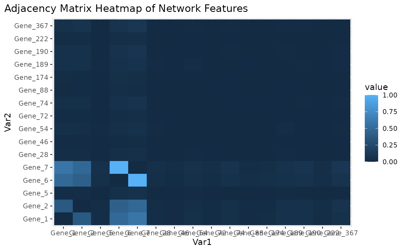
Adjacency matrix heatmap for subnetwork features.

Figure \(\ref{fig:loadings1}\) the visualization of the PC loadings that represents the contribution of each molecular features to the first NetSHy PC. In addition, there are two network heatmaps based on (1) correlation matrix (Figure \(\ref{fig:corheatmap}\)), and (2) adjacency matrix (Figure \(\ref{fig:adjheatmap}\)). Based on the summarization table, genes 1,2,6, and 7 have relatively high correlation with respect to phenotype. The PC loadings also confirm that genes 1,2,5,6,and 7 generally have PC contribution. From the correlation heatmap, we do not observe associations between molecular features, but for the adjacency matrix heatmap, we observe the higher connections between genes 1,2,6, and 7.

Step VI: Visualize network module

The initial approach to network visualization is facilitated through our SmCCNet shinyApp, accessible at https://smccnet.shinyapps.io/smccnetnetwork/. Upon obtaining a subnetwork file named ‘size_a_net_b.Rdata’, users can upload it to the shinyApp. The platform provides various adjustable visualization parameters, enabling users to tailor the network visualization to their preferences. In addition, the Shiny application provides other visualization for the subnetworks in addition to the network, which includes principal component loading visualization, correlation heatmap, and subject-level 3D graph.

An alternative way to visualize the final network module, we need to download the Cytoscape software, and use the package RCy3 to visualize the subnetwork generated from the network trimming step. In general, since the network obtained through the PageRank trimming algorithm is densely connected, and some of the edges may be false positive (meaning that two nodes are not associated, but with higher edge values in the adjacency matrix). Therefore, we use the correlation matrix to filter out those weak network edges.

In the network visualization (Figure \(\ref{fig:netPlot}\)), different colored edges denote different directions of the association between two nodes, where red or blue denotes a positive or negative association respectively. The width of the edge represents the connection strength between two nodes.

library(RCy3)
library(igraph)
# load subnetwork data (example, user need to provide the directory)
load('ResultDirectory/size_a_net_b.Rdata')
M <- as.matrix(M)

# correlation matrix for the subnetwork
filter_index <- which(abs(correlation_sub) < 0.05)
M_ind <- ifelse(correlation_sub > 0, 1, -1)
M_adj <- M * M_ind
M_adj[filter_index] <- 0
diag(M_adj) <- 0

# network visualization through cytoscape
graph <- igraph::graph_from_adjacency_matrix(M_adj, mode = 'undirected', 
         weighted = TRUE, diag = TRUE, add.colnames = NULL, add.rownames = NA)

# define network node type and connectivity
V(graph)$type <- sub_type
V(graph)$type
V(graph)$connectivity <- rowSums(abs(M))
V(graph)$connectivity

createNetworkFromIgraph(graph,"single_omics_network")

Trimmed module 1. The strength of the node connections is indicated by the thickness of edges. Red edges and blue edges are for negative and positive connections respectively.

Single-omics SmCCNet for Binary Phenotype

This section provides a tutorial on running the SmCCNet algorithm for a binary phenotype using single-omics data. Given the binary nature of the phenotype, canonical correlation analysis can be applied, but it may pose challenges due to the correlation issues with binary random variables. To address this, we employ Sparse Partial Least Squares Discriminant Analysis (SPLSDA) to modify the SmCCNet algorithm for binary phenotype.

SPLSDA operates with a dual-stage approach aimed at predicting the phenotype. Initially, it treats the binary phenotype as a quantitative variable and applies partial least squares to derive multiple latent factors. Subsequently, these latent factors are used to predict the binary phenotype using logistic regression. The latent factors are then consolidated into a single factor based on the logistic regression coefficient.

Similar to sparse multiple canonical correlation analysis (SmCCA) used in the quantitative phenotype analysis for SmCCNet, a sparsity parameter needs to be tuned. However, for SPLSDA, an increase in the penalty value results in a higher level of sparsity, which is contrary to the CCA-based method implemented in this package. It’s also important to note that this algorithm is designed specifically for binary phenotypes. For users dealing with multi-class phenotypes, a one-versus-all approach can be used to generate networks separately if the multi-class phenotype is not ordinal. Alternatively, if the multi-class phenotype is ordinal, a CCA-based approach can be applied.

Import synthetic dataset with binary phenotype

As an example, we consider a synthetic data set with 500 genes \((X_1)\) expression levels measured for 358 subjects, along with a binarized phenotype \((Y)\) by taking the median of original phenotype as the cutoff, and transforming it into binary variable.

data(ExampleData)
head(X1[ , 1:6])

##          Gene_1   Gene_2   Gene_3   Gene_4   Gene_5   Gene_6
## Samp_1 22.48570 40.35372 31.02575 20.84721 26.69729 30.20545
## Samp_2 37.05885 34.05223 33.48702 23.53146 26.75463 31.73594
## Samp_3 20.53077 31.66962 35.18957 20.95254 25.01883 32.15723
## Samp_4 33.18689 38.48088 18.89710 31.82330 34.04938 38.79989
## Samp_5 28.96198 41.06049 28.49496 18.37449 30.81524 24.00454
## Samp_6 18.05983 29.55471 32.54002 29.68452 26.19996 26.76684

head(Y)

##           Pheno
## Samp_1 235.0674
## Samp_2 253.5450
## Samp_3 234.2050
## Samp_4 281.0354
## Samp_5 245.4478
## Samp_6 189.6231

# binarize quantitative outcome 
Y <- ifelse(Y > median(Y), 1, 0)

Denote the number of features in \(X_1\) as \(p_1\), and the number of subjects as \(n\).

p1 <- ncol(X1)
N <- nrow(X1)
AbarLabel <- colnames(X1)

The parameter setup for this approach mirrors that of SmCCA, and for more specific information, please refer back to the single-omics quantitative phenotype in section 1.

K <- 3 # number of folds in K-fold CV.
s1 <- 0.7 # feature subsampling percentage.
subSamp <- 50 # number of subsamples.
CCcoef <- NULL # unweighted version of SmCCNet.
metric <- 'auc' # evaluation metric to be used.

# create sparsity penalty options.
pen1 <- seq(.1, .9, by = .1)

# set a CV directory.
CVDir <- "Example3foldCV_Binary/" 
pheno <- "Example3foldCV_Binary"
dir.create(CVDir)

Y <- ifelse(Y > median(Y), 1, 0)

Step II: Determine optimal sparsity penalty through cross-validation (optional)

The SPLS package does not include a method for assessing prediction accuracy. Therefore, we utilize the glm() function from the stats package to evaluate the performance of our model. Particularly for SPLSDA, the number of components is an important factor to consider as the goal is to make predictions. In the following example, we select three as the number of components. All other procedures remain identical to those in SmCCA (see single-omics quantitative phenotype vignette).

set.seed(12345) # set random seed.
# save original data into local directory
save(X1, Y, s1, subSamp, pen1, 
     file = paste0(CVDir, "Data.Rdata"))


# define the number of components to be extracted
ncomp <- 3
# split data into k folds
foldIdx <- split(1:N, sample(1:N, K))
for(i in 1:K){
  iIdx <- foldIdx[[i]]
  x1.train <- scale(X1[-iIdx, ])
  yy.train <- Y[-iIdx, ]
  x1.test <- scale(X1[iIdx, ])
  yy.test <- Y[iIdx, ]
  
  if(is.na(min(min(x1.train), min(yy.train), min(x1.test), min(yy.test)))){
    stop("Invalid scaled data.")
  }
  
  subD <- paste0(CVDir, "CV_", i, "/")
  dir.create(subD)
  save(x1.train, yy.train, x1.test, yy.test,
      pen1, p1, 
       file = paste0(subD, "Data.Rdata"))
}

############################################## Running Cross-Validation

# run SmCCA with K-fold cross-validation
suppressWarnings(for (CVidx in 1:K){
  # define evaluation method
  EvalMethod <- 'precision'
  # define and create saving directory
  subD <- paste0(CVDir, "CV_", CVidx, "/")
  load(paste0(subD, "Data.Rdata"))
  dir.create(paste0(subD, "SmCCA/"))

  # create empty vector to store cross-validation accuracy result
  TrainScore <- TestScore <- rep(0, length(pen1))
  for(idx in 1:length(pen1)){
    # define value of penalty
    l1 <- pen1[idx]

    # run SPLS-DA to extract canonical weight
    Ws <- spls::splsda(x = x1.train, y = yy.train, K = ncomp, eta = l1, 
                       kappa=0.5,
                       classifier= 'logistic', scale.x=FALSE)

    # create emtpy matrix to save canonical weights for each subsampling
    weight <- matrix(0,nrow = ncol(x1.train), ncol = ncomp)
    weight[Ws[["A"]],] <- Ws[["W"]]

    # train the latent factor model with logistic regression
    train_data <- data.frame(x = (x1.train %*% weight)[,1:ncomp], 
                             y = as.factor(yy.train))
    test_data <- data.frame(x = (x1.test %*% weight)[,1:ncomp])
    
    logisticFit <- stats::glm(y~., family = 'binomial',data = train_data)
    # make prediction for train/test set
    train_pred <- stats::predict(logisticFit, train_data, type = 'response')
    test_pred <- stats::predict(logisticFit, test_data, type = 'response')
    # specifying which method to use as evaluation metric
    TrainScore[idx] <- classifierEval(obs = yy.train, 
                                      pred = train_pred, 
                                      EvalMethod = metric, print_score = FALSE)
    TestScore[idx] <- classifierEval(obs = yy.test, 
                                      pred = test_pred, 
                                      EvalMethod = metric, print_score = FALSE)
    
  }

  # combine cross-validation results
  DeltaAcc.all <- as.data.frame(cbind(pen1, TrainScore, TestScore))
  DeltaAcc.all$Delta <- abs(DeltaAcc.all$TrainScore - DeltaAcc.all$TestScore)
  colnames(DeltaAcc.all) <- c("l1", "Training Score", "Testing Score", "Delta")
  
  # save cross-validation results to local directory
  write.csv(DeltaAcc.all,
            file = paste0(subD, "SmCCA/SCCA_", subSamp,"_allDeltaCor.csv"))
  
}
)

Step III: Run SPLSDA with pre-selected penalty term

The evaluation metric is maximizing the classification evaluation metric such as testing prediction accuracy or testing AUC score. Currently there are 5 different evaluation metrics to choose from: accuracy, AUC score, precision, recall, and F1 score, with accuracy as the default selection (see multi-omics vignette section 5 for details). The following example employs the penalty term with the greatest testing prediction accuracy to execute the SPLSDA algorithm on the entire dataset.

# save cross-validation result
cv_result <- aggregateCVSingle(CVDir, "SmCCA", NumSubsamp = subSamp, K = 3)

# create directory to save overall result with the best penalty term
plotD <- paste0(CVDir, "Figures/")
saveD <- paste0(CVDir, "Results/")
dataF <- paste0(CVDir, "Data.Rdata")
dir.create(plotD)
dir.create(saveD)
dir.create(dataF)

# specify method (only SmCCA works)
Method = "SmCCA"

for(Method in "SmCCA"){
  # read cross validation result in
  T12 <- read.csv(paste0(CVDir, "Results/", Method, "CVmeanDeltaCors.csv"))
  # determine the optimal penalty term
  pen <- T12[which.max(T12[ ,3]) ,2]
  l1 <- pen;
  system.time({
    # run SPLSDA with optimal penalty term
    Ws <- getRobustWeightsSingleBinary(X1 = X1, Trait = as.matrix(Y), 
                                       Lambda1 = l1, 
                                       s1, SubsamplingNum = subSamp)
   
    # get adjacency matrix
    Abar <- getAbar(Ws, FeatureLabel = AbarLabel[1:p1])
    # save result into local directory
    save(l1, X1, Y, s1, Ws, Abar,
         file = paste0(saveD, Method, K, "foldSamp", subSamp, "_", pen, 
                       ".Rdata"))
  })
  
  
}

After this step, all the other steps are a consistent with single-omics quantitative phenotype example, refer to section 1.4 and 1.5 for more information.

Session info

sessionInfo()

## R version 4.3.3 (2024-02-29)
## Platform: x86_64-pc-linux-gnu (64-bit)
## Running under: Ubuntu 22.04.4 LTS
## 
## Matrix products: default
## BLAS:   /usr/lib/x86_64-linux-gnu/openblas-pthread/libblas.so.3 
## LAPACK: /usr/lib/x86_64-linux-gnu/openblas-pthread/libopenblasp-r0.3.20.so;  LAPACK version 3.10.0
## 
## locale:
##  [1] LC_CTYPE=C.UTF-8       LC_NUMERIC=C           LC_TIME=C.UTF-8       
##  [4] LC_COLLATE=C.UTF-8     LC_MONETARY=C.UTF-8    LC_MESSAGES=C.UTF-8   
##  [7] LC_PAPER=C.UTF-8       LC_NAME=C              LC_ADDRESS=C          
## [10] LC_TELEPHONE=C         LC_MEASUREMENT=C.UTF-8 LC_IDENTIFICATION=C   
## 
## time zone: UTC
## tzcode source: system (glibc)
## 
## attached base packages:
## [1] grid      parallel  stats     graphics  grDevices utils     datasets 
## [8] methods   base     
## 
## other attached packages:
##  [1] reshape2_1.4.4   shadowtext_0.1.3 lubridate_1.9.3  forcats_1.0.0   
##  [5] stringr_1.5.1    dplyr_1.1.4      purrr_1.0.2      readr_2.1.5     
##  [9] tidyr_1.3.1      tibble_3.2.1     ggplot2_3.5.0    tidyverse_2.0.0 
## [13] SmCCNet_2.0.3    igraph_2.0.3     Matrix_1.6-5     pbapply_1.7-2   
## 
## loaded via a namespace (and not attached):
##  [1] sass_0.4.9        utf8_1.2.4        generics_0.1.3    stringi_1.8.3    
##  [5] lattice_0.22-5    hms_1.1.3         digest_0.6.35     magrittr_2.0.3   
##  [9] timechange_0.3.0  evaluate_0.23     fastmap_1.1.1     plyr_1.8.9       
## [13] jsonlite_1.8.8    fansi_1.0.6       scales_1.3.0      textshaping_0.3.7
## [17] jquerylib_0.1.4   cli_3.6.2         rlang_1.1.3       munsell_0.5.1    
## [21] withr_3.0.0       cachem_1.0.8      yaml_2.3.8        tools_4.3.3      
## [25] tzdb_0.4.0        memoise_2.0.1     colorspace_2.1-0  vctrs_0.6.5      
## [29] R6_2.5.1          lifecycle_1.0.4   fs_1.6.3          ragg_1.3.0       
## [33] pkgconfig_2.0.3   desc_1.4.3        pkgdown_2.0.8     bslib_0.7.0      
## [37] pillar_1.9.0      gtable_0.3.4      Rcpp_1.0.12       glue_1.7.0       
## [41] systemfonts_1.0.6 xfun_0.43         tidyselect_1.2.1  highr_0.10       
## [45] knitr_1.46        farver_2.1.1      htmltools_0.5.8.1 labeling_0.4.3   
## [49] rmarkdown_2.26    compiler_4.3.3

warnings()

References

Shi, W. J., Zhuang, Y., Russell, P. H., Hobbs, B. D., Parker, M. M., Castaldi, P. J., … & Kechris, K. (2019). Unsupervised discovery of phenotype-specific multi-omics networks. Bioinformatics, 35(21), 4336-4343.

Vu, T., Litkowski, E. M., Liu, W., Pratte, K. A., Lange, L., Bowler, R. P., … & Kechris, K. J. (2023). NetSHy: network summarization via a hybrid approach leveraging topological properties. Bioinformatics, 39(1), btac818.

Weixuan Liu

Katerina Kechris

2024-04-16